Visualize dynophores: Point clouds in 3D
In this notebook, we will show how to view the dynophore point clouds in 3D using nglview.
[1]:
%load_ext autoreload
%autoreload 2
[2]:
from pathlib import Path

from dynophores import Dynophore
from dynophores import view3d
Set paths to data files
[3]:
DATA = Path("../../dynophores/tests/data")
dyno_path = DATA / "out"
pdb_path = DATA / "in/startframe.pdb"
dcd_path = DATA / "in/trajectory.dcd"
Load data as Dynophore object
[4]:
dynophore = Dynophore.from_dir(dyno_path)
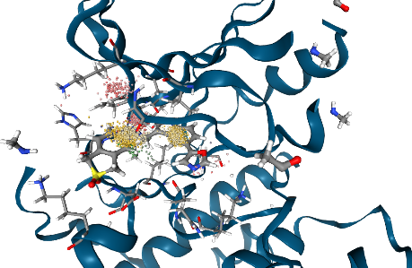
Show structure with dynophore
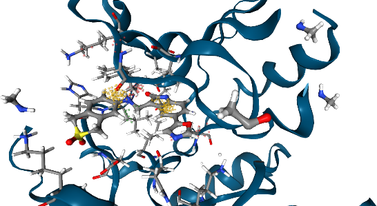
Let’s visualize the 3D dynophore alongside an example macromolecule-ligand conformation from the MD simulation (start frame).
[5]:
view = view3d.show(dynophore, pdb_path, visualization_type="spheres")  # Spheres are the default
view.display(gui=True, style="ngl")
[8]:
view.render_image(trim=True, factor=1, transparent=True);
[9]:
view._display_image()
[9]:
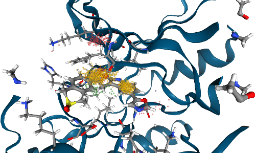
Using the NGL GUI, you can toggle on/off the pocket side chain residues that are interacting with the ligand.
[10]:
view = view3d.show(dynophore, pdb_path, visualization_type="spheres")
view.display(gui=True, style="ngl")
[11]:
view.render_image(trim=True, factor=1, transparent=True);
[12]:
view._display_image()
[12]:
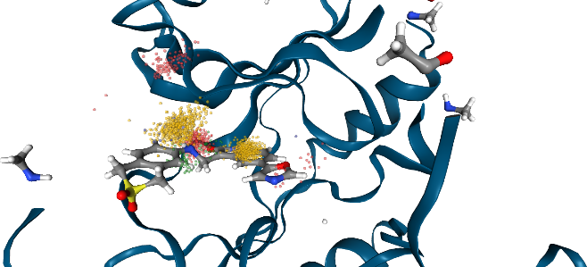
By nature, this (static) structure cannot rationalize some of the (dynamic) dynophore point clouds. So let’s use the trajectory instead.
Show trajectory with dynophore
Let’s visualize the 3D dynophore alongside the macromolecule-ligand trajectory.
[13]:
view = view3d.show(dynophore, pdb_path, dcd_path)
view.display(gui=True, style="ngl")
[14]:
view.render_image(trim=True, factor=1, transparent=True);
[15]:
view._display_image()
[15]:
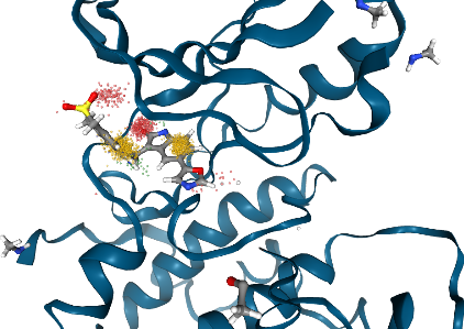
Show dynophore with frame resolution
[16]:
view = view3d.show(dynophore, pdb_path, visualization_type="spheres", color_cloud_by_frame=True)
view.display(gui=True, style="ngl")
[17]:
view.render_image(trim=True, factor=1, transparent=True);
[18]:
view._display_image()
[18]:
Show dynophore for selected frame range
[19]:
view = view3d.show(dynophore, pdb_path, visualization_type="spheres", frame_range=[900, 1000])
view.display(gui=True, style="ngl")
[20]:
view.render_image(trim=True, factor=1, transparent=True);
[21]:
view._display_image()
[21]: